Introduction dvb.datascience
In this tutorial, you will learn what the basic usage of dvb.datascience is and how you can use in in your datascience activities.
If you have any suggestions for features or if you encounter any bugs, please let us know at tc@devolksbank.nl
In [1]:
# %matplotlib inline
import dvb.datascience as ds
Defining a pipeline
Defining a pipeline is just adding some Pipes (actions) which will be connected
Every Pipe can have 0, 1 or more inputs from other pipes. Every Pipe can have 0, 1 or more outputs to other pipes. Every Pipe has a name. Every input and output of the pipe has a key by which the input/output is identified. The name of the Pipe and the key of the input/output are used to connect pipes.
In [2]:
p = ds.Pipeline()
p.addPipe("read", ds.data.SampleData(dataset_name="iris"))
p.addPipe("metadata", ds.data.DataPipe("df_metadata", {"y_true_label": "label"}))
p.addPipe("write",ds.data.CSVDataExportPipe("dump_input_to_output.csv", sep=",", index_label="caseId"),[("read", "df", "df")],)
Out[2]:
<dvb.datascience.pipeline.Pipeline at 0x7f84803bd400>
A pipeline has two main methods: fit_transform() and
transform().fit_transform() is training the pipeline. Depending on
the Pipe, the training can be computing the mean, making a decision
tree, etc. During the transform, those learnings are used to transform()
the input to output, for example by replacing outliers by means,
predicting with the trained model, etc.
In [3]:
p.fit_transform()
'Drawing diagram using blockdiag'
<PIL.PngImagePlugin.PngImageFile image mode=RGB size=448x280 at 0x7F84802D7198>
Transform fit
After the transform, the output of the transform is available.
In [4]:
p.get_pipe_output('read')
Out[4]:
{'df':      sepal length (cm)  sepal width (cm)  petal length (cm)  petal width (cm)  \
 0                  5.1               3.5                1.4               0.2
 1                  4.9               3.0                1.4               0.2
 2                  4.7               3.2                1.3               0.2
 3                  4.6               3.1                1.5               0.2
 4                  5.0               3.6                1.4               0.2
 5                  5.4               3.9                1.7               0.4
 6                  4.6               3.4                1.4               0.3
 7                  5.0               3.4                1.5               0.2
 8                  4.4               2.9                1.4               0.2
 9                  4.9               3.1                1.5               0.1
 10                 5.4               3.7                1.5               0.2
 11                 4.8               3.4                1.6               0.2
 12                 4.8               3.0                1.4               0.1
 13                 4.3               3.0                1.1               0.1
 14                 5.8               4.0                1.2               0.2
 15                 5.7               4.4                1.5               0.4
 16                 5.4               3.9                1.3               0.4
 17                 5.1               3.5                1.4               0.3
 18                 5.7               3.8                1.7               0.3
 19                 5.1               3.8                1.5               0.3
 20                 5.4               3.4                1.7               0.2
 21                 5.1               3.7                1.5               0.4
 22                 4.6               3.6                1.0               0.2
 23                 5.1               3.3                1.7               0.5
 24                 4.8               3.4                1.9               0.2
 25                 5.0               3.0                1.6               0.2
 26                 5.0               3.4                1.6               0.4
 27                 5.2               3.5                1.5               0.2
 28                 5.2               3.4                1.4               0.2
 29                 4.7               3.2                1.6               0.2
 ..                 ...               ...                ...               ...
 120                6.9               3.2                5.7               2.3
 121                5.6               2.8                4.9               2.0
 122                7.7               2.8                6.7               2.0
 123                6.3               2.7                4.9               1.8
 124                6.7               3.3                5.7               2.1
 125                7.2               3.2                6.0               1.8
 126                6.2               2.8                4.8               1.8
 127                6.1               3.0                4.9               1.8
 128                6.4               2.8                5.6               2.1
 129                7.2               3.0                5.8               1.6
 130                7.4               2.8                6.1               1.9
 131                7.9               3.8                6.4               2.0
 132                6.4               2.8                5.6               2.2
 133                6.3               2.8                5.1               1.5
 134                6.1               2.6                5.6               1.4
 135                7.7               3.0                6.1               2.3
 136                6.3               3.4                5.6               2.4
 137                6.4               3.1                5.5               1.8
 138                6.0               3.0                4.8               1.8
 139                6.9               3.1                5.4               2.1
 140                6.7               3.1                5.6               2.4
 141                6.9               3.1                5.1               2.3
 142                5.8               2.7                5.1               1.9
 143                6.8               3.2                5.9               2.3
 144                6.7               3.3                5.7               2.5
 145                6.7               3.0                5.2               2.3
 146                6.3               2.5                5.0               1.9
 147                6.5               3.0                5.2               2.0
 148                6.2               3.4                5.4               2.3
 149                5.9               3.0                5.1               1.8

      target
 0         0
 1         0
 2         0
 3         0
 4         0
 5         0
 6         0
 7         0
 8         0
 9         0
 10        0
 11        0
 12        0
 13        0
 14        0
 15        0
 16        0
 17        0
 18        0
 19        0
 20        0
 21        0
 22        0
 23        0
 24        0
 25        0
 26        0
 27        0
 28        0
 29        0
 ..      ...
 120       2
 121       2
 122       2
 123       2
 124       2
 125       2
 126       2
 127       2
 128       2
 129       2
 130       2
 131       2
 132       2
 133       2
 134       2
 135       2
 136       2
 137       2
 138       2
 139       2
 140       2
 141       2
 142       2
 143       2
 144       2
 145       2
 146       2
 147       2
 148       2
 149       2

 [150 rows x 5 columns],
 'df_metadata': {'classes': ['Setosa', 'Versicolour', 'Virginica'],
  'y_true_label': 'target'},
 'y_names': array(['setosa', 'versicolor', 'virginica'], dtype='<U10')}
Multiple inputs
Some Pipes have multiple inputs, for example to merge two datasets we can do the following.
In [5]:
p = ds.Pipeline()
p.addPipe('read1', ds.data.CSVDataImportPipe())
p.addPipe('read2', ds.data.CSVDataImportPipe())
p.addPipe('merge', ds.transform.Union(2, axis=0, join='outer'), [("read1", "df", "df0"), ("read2", "df", "df1")])
Out[5]:
<dvb.datascience.pipeline.Pipeline at 0x7f847fb1c128>
In [6]:
p.fit_transform(transform_params={'read1': {'file_path': '../test/data/train.csv'}, 'read2': {'file_path': '../test/data/test.csv'}})
'Drawing diagram using blockdiag'
<PIL.PngImagePlugin.PngImageFile image mode=RGB size=448x280 at 0x7F847FB379B0>
Transform fit
In [7]:
p.get_pipe_output('merge')
Out[7]:
{'df':    age gender  length   name
 0   20      M     180    jan
 1   21      W     164  marie
 2   23      M     194   piet
 3   24      W     177  helen
 4   60      U     188    jan
 0   25      W     161    gea
 1   65      M     181   marc}
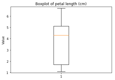
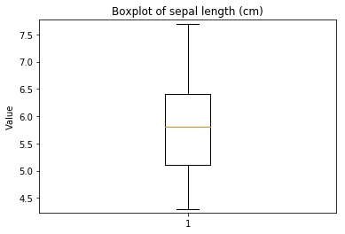
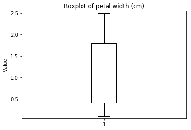
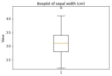
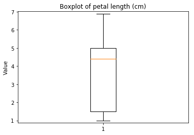
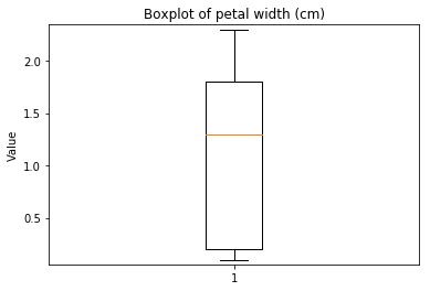
Plots
It’s easy to get some plots of the data:
In [8]:
p = ds.Pipeline()
p.addPipe('read', ds.data.SampleData('iris'))
p.addPipe('split', ds.transform.RandomTrainTestSplit(test_size=0.3), [("read", "df", "df")])
p.addPipe('boxplot', ds.eda.BoxPlot(), [("split", "df", "df")])
p.fit_transform(transform_params={'split': {'split': ds.transform.split.TrainTestSplitBase.TRAIN}})
'Drawing diagram using blockdiag'
<PIL.PngImagePlugin.PngImageFile image mode=RGB size=256x360 at 0x7F847FB1CB70>
Transform fit
Boxplots Transform fit


In [9]:
p.get_pipe_output('read')
Out[9]:
{'df':      sepal length (cm)  sepal width (cm)  petal length (cm)  petal width (cm)  \
 0                  5.1               3.5                1.4               0.2
 1                  4.9               3.0                1.4               0.2
 2                  4.7               3.2                1.3               0.2
 3                  4.6               3.1                1.5               0.2
 4                  5.0               3.6                1.4               0.2
 5                  5.4               3.9                1.7               0.4
 6                  4.6               3.4                1.4               0.3
 7                  5.0               3.4                1.5               0.2
 8                  4.4               2.9                1.4               0.2
 9                  4.9               3.1                1.5               0.1
 10                 5.4               3.7                1.5               0.2
 11                 4.8               3.4                1.6               0.2
 12                 4.8               3.0                1.4               0.1
 13                 4.3               3.0                1.1               0.1
 14                 5.8               4.0                1.2               0.2
 15                 5.7               4.4                1.5               0.4
 16                 5.4               3.9                1.3               0.4
 17                 5.1               3.5                1.4               0.3
 18                 5.7               3.8                1.7               0.3
 19                 5.1               3.8                1.5               0.3
 20                 5.4               3.4                1.7               0.2
 21                 5.1               3.7                1.5               0.4
 22                 4.6               3.6                1.0               0.2
 23                 5.1               3.3                1.7               0.5
 24                 4.8               3.4                1.9               0.2
 25                 5.0               3.0                1.6               0.2
 26                 5.0               3.4                1.6               0.4
 27                 5.2               3.5                1.5               0.2
 28                 5.2               3.4                1.4               0.2
 29                 4.7               3.2                1.6               0.2
 ..                 ...               ...                ...               ...
 120                6.9               3.2                5.7               2.3
 121                5.6               2.8                4.9               2.0
 122                7.7               2.8                6.7               2.0
 123                6.3               2.7                4.9               1.8
 124                6.7               3.3                5.7               2.1
 125                7.2               3.2                6.0               1.8
 126                6.2               2.8                4.8               1.8
 127                6.1               3.0                4.9               1.8
 128                6.4               2.8                5.6               2.1
 129                7.2               3.0                5.8               1.6
 130                7.4               2.8                6.1               1.9
 131                7.9               3.8                6.4               2.0
 132                6.4               2.8                5.6               2.2
 133                6.3               2.8                5.1               1.5
 134                6.1               2.6                5.6               1.4
 135                7.7               3.0                6.1               2.3
 136                6.3               3.4                5.6               2.4
 137                6.4               3.1                5.5               1.8
 138                6.0               3.0                4.8               1.8
 139                6.9               3.1                5.4               2.1
 140                6.7               3.1                5.6               2.4
 141                6.9               3.1                5.1               2.3
 142                5.8               2.7                5.1               1.9
 143                6.8               3.2                5.9               2.3
 144                6.7               3.3                5.7               2.5
 145                6.7               3.0                5.2               2.3
 146                6.3               2.5                5.0               1.9
 147                6.5               3.0                5.2               2.0
 148                6.2               3.4                5.4               2.3
 149                5.9               3.0                5.1               1.8

      target
 0         0
 1         0
 2         0
 3         0
 4         0
 5         0
 6         0
 7         0
 8         0
 9         0
 10        0
 11        0
 12        0
 13        0
 14        0
 15        0
 16        0
 17        0
 18        0
 19        0
 20        0
 21        0
 22        0
 23        0
 24        0
 25        0
 26        0
 27        0
 28        0
 29        0
 ..      ...
 120       2
 121       2
 122       2
 123       2
 124       2
 125       2
 126       2
 127       2
 128       2
 129       2
 130       2
 131       2
 132       2
 133       2
 134       2
 135       2
 136       2
 137       2
 138       2
 139       2
 140       2
 141       2
 142       2
 143       2
 144       2
 145       2
 146       2
 147       2
 148       2
 149       2

 [150 rows x 5 columns],
 'df_metadata': {'classes': ['Setosa', 'Versicolour', 'Virginica'],
  'y_true_label': 'target'},
 'y_names': array(['setosa', 'versicolor', 'virginica'], dtype='<U10')}
In [10]:
p.transform(transform_params={'split': {'split': ds.transform.split.TrainTestSplitBase.TEST}}, name='test', close_plt=True)
'Drawing diagram using blockdiag'
<PIL.PngImagePlugin.PngImageFile image mode=RGB size=256x360 at 0x7F847D8E2518>
Transform test
Boxplots Transform test


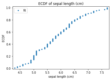
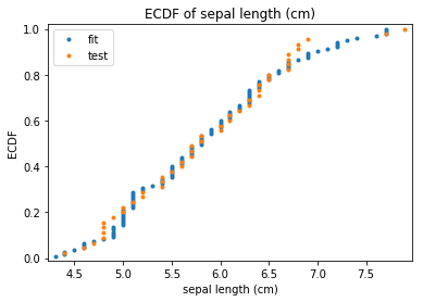
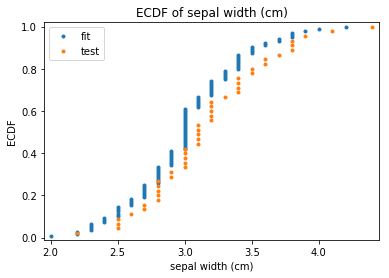
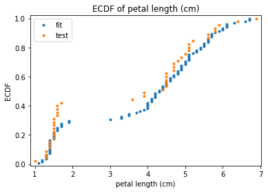
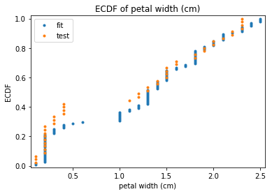
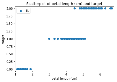
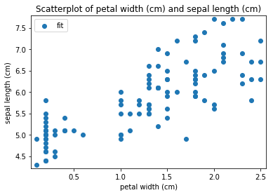
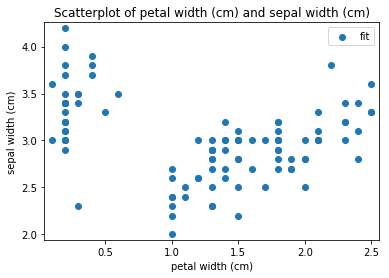
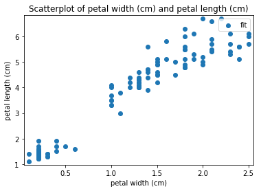
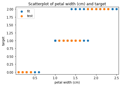
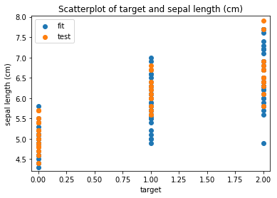
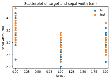
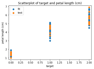
Some plots can combine transforms to one plot
You can add a name to the transform in order to add it to the legend. By default, the transform won’t close the plots. So when you leave out close_plt=True in the call of (fit_)transform, plots of the next transform will be integrated in the plots of the previous transform. Do not forget to call close_plt=True on the last transform, otherwise all plots will remain open and will be plotted by jupyter again.
In [11]:
p = ds.Pipeline()
p.addPipe('read', ds.data.SampleData('iris'))
p.addPipe('split', ds.transform.RandomTrainTestSplit(test_size=0.3), [("read", "df", "df")])
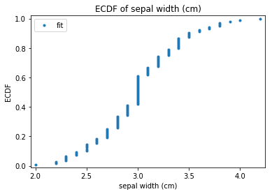
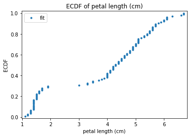
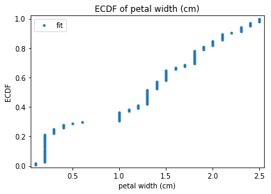
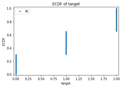
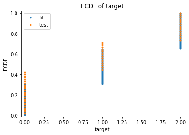
p.addPipe('ecdf', ds.eda.ECDFPlots(), [("split", "df", "df")])
p.fit_transform(transform_params={'split': {'split': ds.transform.split.TrainTestSplitBase.TRAIN}})
p.transform(transform_params={'split': {'split': ds.transform.split.TrainTestSplitBase.TEST}}, name='test', close_plt=True)
'Drawing diagram using blockdiag'
<PIL.PngImagePlugin.PngImageFile image mode=RGB size=256x360 at 0x7F847FB39C50>
Transform fit
ECDF Plots Transform fit
'Drawing diagram using blockdiag'
<PIL.PngImagePlugin.PngImageFile image mode=RGB size=256x360 at 0x7F847D51C4E0>
Transform test
ECDF Plots Transform test
In [12]:
p = ds.Pipeline()
p.addPipe('read', ds.data.SampleData('iris'))
p.addPipe('split', ds.transform.RandomTrainTestSplit(test_size=0.3), [("read", "df", "df")])
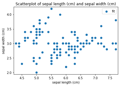
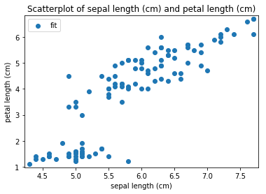
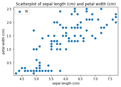
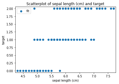
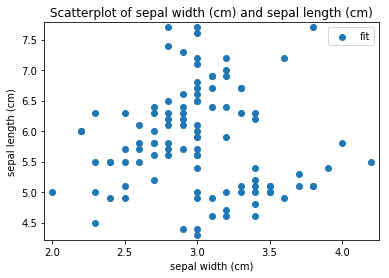
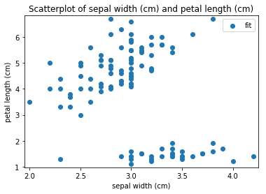
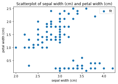
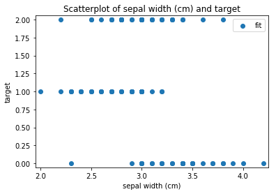
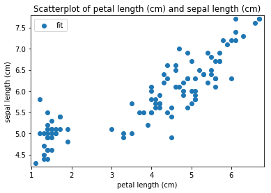
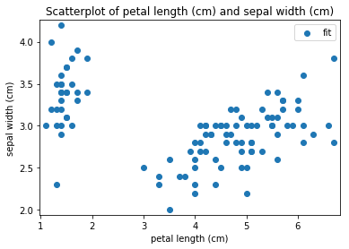
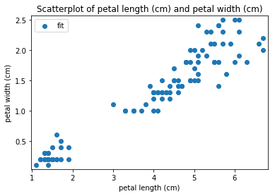
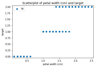
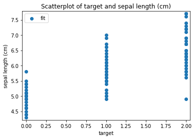
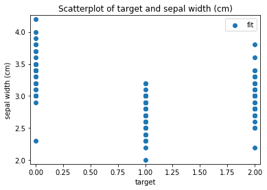
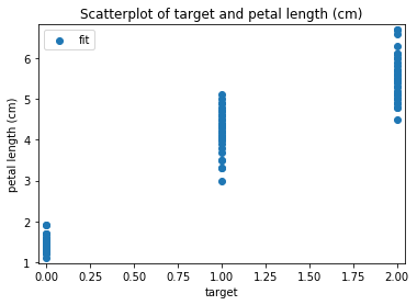
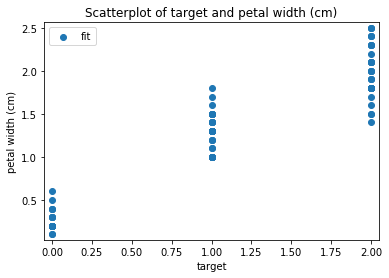
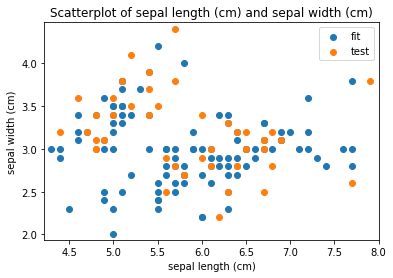
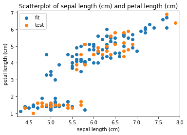
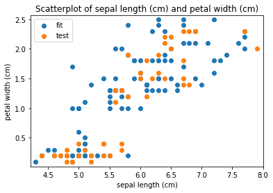
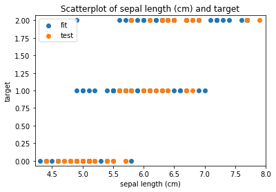
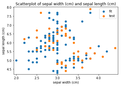
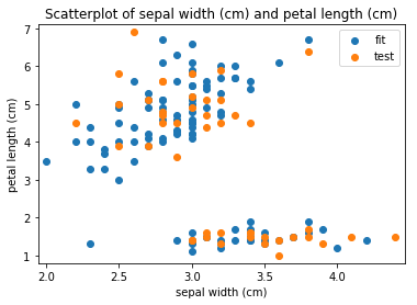
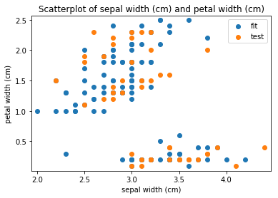
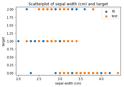
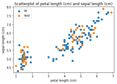
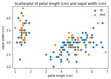
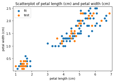
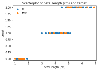
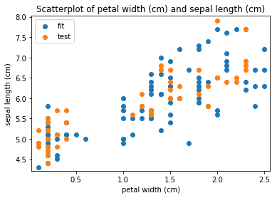
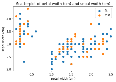
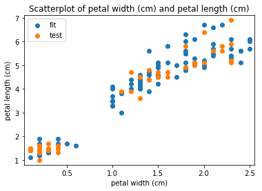
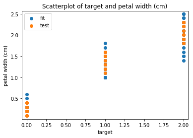
p.addPipe('scatter', ds.eda.ScatterPlots(), [("split", "df", "df")])
p.fit_transform(transform_params={'split': {'split': ds.transform.split.TrainTestSplitBase.TRAIN}})
p.transform(transform_params={'split': {'split': ds.transform.split.TrainTestSplitBase.TEST}}, name='test', close_plt=True)
'Drawing diagram using blockdiag'
<PIL.PngImagePlugin.PngImageFile image mode=RGB size=256x360 at 0x7F847D7452B0>
Transform fit
Scatterplots Transform fit
'Drawing diagram using blockdiag'
<PIL.PngImagePlugin.PngImageFile image mode=RGB size=256x360 at 0x7F847D74F400>
Transform test
Scatterplots Transform test
In [13]:
p = ds.Pipeline()
p.addPipe('read', ds.data.SampleData('iris'))
p.addPipe('split', ds.transform.RandomTrainTestSplit(test_size=0.3), [("read", "df", "df")])
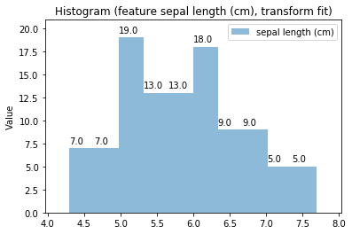
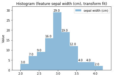
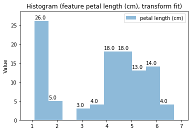
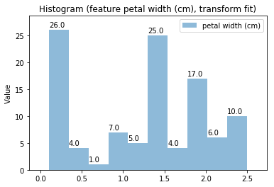
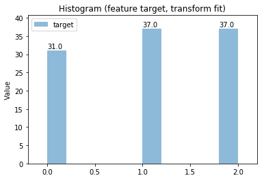
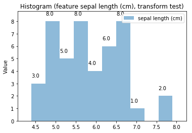
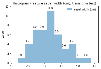
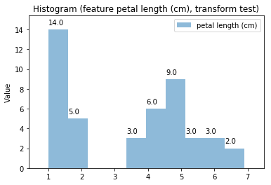
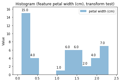
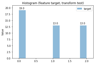
p.addPipe('hist', ds.eda.Hist(), [("split", "df", "df")])
p.fit_transform(transform_params={'split': {'split': ds.transform.split.TrainTestSplitBase.TRAIN}})
p.transform(transform_params={'split': {'split': ds.transform.split.TrainTestSplitBase.TEST}}, name='test', close_plt=True)
'Drawing diagram using blockdiag'
<PIL.PngImagePlugin.PngImageFile image mode=RGB size=256x360 at 0x7F847D430F60>
Transform fit
Histogram Transform fit
'Drawing diagram using blockdiag'
<PIL.PngImagePlugin.PngImageFile image mode=RGB size=256x360 at 0x7F847CF17978>
Transform test
Histogram Transform test
Drawing a pipeline
Once defined, a pipeline can be drawn.
In [14]:
p = ds.Pipeline()
p.addPipe('read', ds.data.CSVDataImportPipe())
p.addPipe('read2', ds.data.CSVDataImportPipe())
p.addPipe('numeric', ds.transform.FilterTypeFeatures(), [("read", "df", "df")])
p.addPipe('numeric2', ds.transform.FilterTypeFeatures(), [("read2", "df", "df")])
p.addPipe('boxplot', ds.eda.BoxPlot(), [("numeric", "df", "df"), ("numeric2", "df", "df")])
p.draw_design()
'Drawing diagram using blockdiag'
<PIL.PngImagePlugin.PngImageFile image mode=RGB size=448x360 at 0x7F847D9F4048>
Predicting
In [15]:
from sklearn.neighbors import KNeighborsClassifier
p = ds.Pipeline()
p.addPipe('read', ds.data.SampleData('iris'))
p.addPipe('clf', ds.predictor.SklearnClassifier(KNeighborsClassifier, n_neighbors=3), [("read", "df", "df"), ("read", "df_metadata", "df_metadata")])
p.fit_transform()
p.get_pipe_output('clf')
'Drawing diagram using blockdiag'
<PIL.PngImagePlugin.PngImageFile image mode=RGB size=256x280 at 0x7F847CCC5550>
Transform fit
Out[15]:
{'predict':      y_pred_Setosa  y_pred_Versicolour  y_pred_Virginica  y_pred  target
 0              1.0            0.000000          0.000000     0.0       0
 1              1.0            0.000000          0.000000     0.0       0
 2              1.0            0.000000          0.000000     0.0       0
 3              1.0            0.000000          0.000000     0.0       0
 4              1.0            0.000000          0.000000     0.0       0
 5              1.0            0.000000          0.000000     0.0       0
 6              1.0            0.000000          0.000000     0.0       0
 7              1.0            0.000000          0.000000     0.0       0
 8              1.0            0.000000          0.000000     0.0       0
 9              1.0            0.000000          0.000000     0.0       0
 10             1.0            0.000000          0.000000     0.0       0
 11             1.0            0.000000          0.000000     0.0       0
 12             1.0            0.000000          0.000000     0.0       0
 13             1.0            0.000000          0.000000     0.0       0
 14             1.0            0.000000          0.000000     0.0       0
 15             1.0            0.000000          0.000000     0.0       0
 16             1.0            0.000000          0.000000     0.0       0
 17             1.0            0.000000          0.000000     0.0       0
 18             1.0            0.000000          0.000000     0.0       0
 19             1.0            0.000000          0.000000     0.0       0
 20             1.0            0.000000          0.000000     0.0       0
 21             1.0            0.000000          0.000000     0.0       0
 22             1.0            0.000000          0.000000     0.0       0
 23             1.0            0.000000          0.000000     0.0       0
 24             1.0            0.000000          0.000000     0.0       0
 25             1.0            0.000000          0.000000     0.0       0
 26             1.0            0.000000          0.000000     0.0       0
 27             1.0            0.000000          0.000000     0.0       0
 28             1.0            0.000000          0.000000     0.0       0
 29             1.0            0.000000          0.000000     0.0       0
 ..             ...                 ...               ...     ...     ...
 120            0.0            0.000000          1.000000     0.0       2
 121            0.0            0.000000          1.000000     0.0       2
 122            0.0            0.000000          1.000000     0.0       2
 123            0.0            0.000000          1.000000     0.0       2
 124            0.0            0.000000          1.000000     0.0       2
 125            0.0            0.000000          1.000000     0.0       2
 126            0.0            0.000000          1.000000     0.0       2
 127            0.0            0.000000          1.000000     0.0       2
 128            0.0            0.000000          1.000000     0.0       2
 129            0.0            0.000000          1.000000     0.0       2
 130            0.0            0.000000          1.000000     0.0       2
 131            0.0            0.000000          1.000000     0.0       2
 132            0.0            0.000000          1.000000     0.0       2
 133            0.0            0.666667          0.333333     1.0       2
 134            0.0            0.333333          0.666667     0.0       2
 135            0.0            0.000000          1.000000     0.0       2
 136            0.0            0.000000          1.000000     0.0       2
 137            0.0            0.000000          1.000000     0.0       2
 138            0.0            0.333333          0.666667     0.0       2
 139            0.0            0.000000          1.000000     0.0       2
 140            0.0            0.000000          1.000000     0.0       2
 141            0.0            0.000000          1.000000     0.0       2
 142            0.0            0.000000          1.000000     0.0       2
 143            0.0            0.000000          1.000000     0.0       2
 144            0.0            0.000000          1.000000     0.0       2
 145            0.0            0.000000          1.000000     0.0       2
 146            0.0            0.000000          1.000000     0.0       2
 147            0.0            0.000000          1.000000     0.0       2
 148            0.0            0.000000          1.000000     0.0       2
 149            0.0            0.000000          1.000000     0.0       2

 [150 rows x 5 columns],
 'predict_metadata': {'classes': ['Setosa', 'Versicolour', 'Virginica'],
  'y_true_label': 'target',
  'threshold': 0.5}}
Scoring
In [16]:
from sklearn.neighbors import KNeighborsClassifier
p = ds.Pipeline()
p.addPipe('read', ds.data.SampleData('iris'))
p.addPipe('clf', ds.predictor.SklearnClassifier(KNeighborsClassifier, n_neighbors=3), [("read", "df", "df"), ("read", "df_metadata", "df_metadata")])
p.addPipe('score', ds.score.ClassificationScore(), [("clf", "predict", "predict"), ("clf", "predict_metadata", "predict_metadata")])
p.fit_transform()
'Drawing diagram using blockdiag'
<PIL.PngImagePlugin.PngImageFile image mode=RGB size=256x360 at 0x7F847D752400>
Transform fit
'auc() not yet implemented for multiclass classifiers'
'plot_auc() not yet implemented for multiclass classifiers'
accuracy
| fit |
|---|
| 0.646667 |
mcc
| fit |
|---|
| 0.57563 |
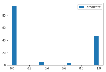
Confusion Matrix

'Precision-recall-curve not yet implemented for multiclass classifiers'
'log_loss() not yet implemented for multiclass classifiers'
Classification Report
/home/docs/checkouts/readthedocs.org/user_builds/dvb-datascience-test/envs/latest/lib/python3.6/site-packages/sklearn/metrics/classification.py:1143: UndefinedMetricWarning: Precision and F-score are ill-defined and being set to 0.0 in labels with no predicted samples.
  'precision', 'predicted', average, warn_for)
| precision | recall | f1-score | support | |
|---|---|---|---|---|
| Setosa | 0.50 | 1.00 | 0.666667 | 50.0 |
| Versicolour | 0.94 | 0.94 | 0.940000 | 50.0 |
| Virginica | 0.00 | 0.00 | 0.000000 | 50.0 |
| avg/total | 0.48 | 0.65 | 0.540000 | 150.0 |
Model Performance


Fetching the output
You can fetch the output of a pipe using the following:
In [17]:
p.get_pipe_output('clf')
Out[17]:
{'predict':      y_pred_Setosa  y_pred_Versicolour  y_pred_Virginica  y_pred  target
 0              1.0            0.000000          0.000000     0.0       0
 1              1.0            0.000000          0.000000     0.0       0
 2              1.0            0.000000          0.000000     0.0       0
 3              1.0            0.000000          0.000000     0.0       0
 4              1.0            0.000000          0.000000     0.0       0
 5              1.0            0.000000          0.000000     0.0       0
 6              1.0            0.000000          0.000000     0.0       0
 7              1.0            0.000000          0.000000     0.0       0
 8              1.0            0.000000          0.000000     0.0       0
 9              1.0            0.000000          0.000000     0.0       0
 10             1.0            0.000000          0.000000     0.0       0
 11             1.0            0.000000          0.000000     0.0       0
 12             1.0            0.000000          0.000000     0.0       0
 13             1.0            0.000000          0.000000     0.0       0
 14             1.0            0.000000          0.000000     0.0       0
 15             1.0            0.000000          0.000000     0.0       0
 16             1.0            0.000000          0.000000     0.0       0
 17             1.0            0.000000          0.000000     0.0       0
 18             1.0            0.000000          0.000000     0.0       0
 19             1.0            0.000000          0.000000     0.0       0
 20             1.0            0.000000          0.000000     0.0       0
 21             1.0            0.000000          0.000000     0.0       0
 22             1.0            0.000000          0.000000     0.0       0
 23             1.0            0.000000          0.000000     0.0       0
 24             1.0            0.000000          0.000000     0.0       0
 25             1.0            0.000000          0.000000     0.0       0
 26             1.0            0.000000          0.000000     0.0       0
 27             1.0            0.000000          0.000000     0.0       0
 28             1.0            0.000000          0.000000     0.0       0
 29             1.0            0.000000          0.000000     0.0       0
 ..             ...                 ...               ...     ...     ...
 120            0.0            0.000000          1.000000     0.0       2
 121            0.0            0.000000          1.000000     0.0       2
 122            0.0            0.000000          1.000000     0.0       2
 123            0.0            0.000000          1.000000     0.0       2
 124            0.0            0.000000          1.000000     0.0       2
 125            0.0            0.000000          1.000000     0.0       2
 126            0.0            0.000000          1.000000     0.0       2
 127            0.0            0.000000          1.000000     0.0       2
 128            0.0            0.000000          1.000000     0.0       2
 129            0.0            0.000000          1.000000     0.0       2
 130            0.0            0.000000          1.000000     0.0       2
 131            0.0            0.000000          1.000000     0.0       2
 132            0.0            0.000000          1.000000     0.0       2
 133            0.0            0.666667          0.333333     1.0       2
 134            0.0            0.333333          0.666667     0.0       2
 135            0.0            0.000000          1.000000     0.0       2
 136            0.0            0.000000          1.000000     0.0       2
 137            0.0            0.000000          1.000000     0.0       2
 138            0.0            0.333333          0.666667     0.0       2
 139            0.0            0.000000          1.000000     0.0       2
 140            0.0            0.000000          1.000000     0.0       2
 141            0.0            0.000000          1.000000     0.0       2
 142            0.0            0.000000          1.000000     0.0       2
 143            0.0            0.000000          1.000000     0.0       2
 144            0.0            0.000000          1.000000     0.0       2
 145            0.0            0.000000          1.000000     0.0       2
 146            0.0            0.000000          1.000000     0.0       2
 147            0.0            0.000000          1.000000     0.0       2
 148            0.0            0.000000          1.000000     0.0       2
 149            0.0            0.000000          1.000000     0.0       2

 [150 rows x 5 columns],
 'predict_metadata': {'classes': ['Setosa', 'Versicolour', 'Virginica'],
  'y_true_label': 'target',
  'threshold': 0.5}}
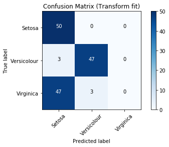
Confusion matrix
You can print the confusion matrix of a score pipe using the following:
In [18]:
p.get_pipe('score').plot_confusion_matrix()
Confusion Matrix

Out[18]:

Precision Recall Curve
And the same holds for the precision recall curve:
In [19]:
p.get_pipe('score').precision_recall_curve()
'Precision-recall-curve not yet implemented for multiclass classifiers'
AUC plot
As well as the AUC plot
In [20]:
p.get_pipe('score').plot_auc()
'plot_auc() not yet implemented for multiclass classifiers'